Intro

Beam SQL allows a Beam user to query PCollections with SQL statements. Interactive Beam provides an integration between Apache Beam and Jupyter Notebooks (formerly known as IPython Notebooks) to make pipeline prototyping and data exploration much faster and easier. You can set up your own notebook user interface (for example, JupyterLab or classic Jupyter Notebooks) on your own device following their documentations. Alternatively, you can choose a hosted solution that does everything for you. You are free to select whichever notebook user interface you prefer. For simplicity, this post does not go through the notebook environment setup and uses Apache Beam Notebooks that provides a cloud-hosted JupyterLab environment and lets a Beam user iteratively develop pipelines, inspect pipeline graphs, and parse individual PCollections in a read-eval-print-loop (REPL) workflow.

In this post, you will see how to use beam_sql, a notebook magic, to execute Beam SQL in notebooks and inspect the results.

By the end of the post, it also demonstrates how to use the beam_sql magic with a production environment, such as running it as a one-shot job on Dataflow. It’s optional. To follow those steps, you should have a project in Google Cloud Platform with necessary APIs enabled , and you should have enough permissions to create a Google Cloud Storage bucket (or to use an existing one), query a public Google Cloud BigQuery dataset, and run Dataflow jobs.

If you choose to use the cloud hosted notebook solution, once you have your Google Cloud project ready, you will need to create an Apache Beam Notebooks instance and open the JupyterLab web interface. Please follow the instructions given at: https://cloud.google.com/dataflow/docs/guides/interactive-pipeline-development#launching_an_notebooks_instance

Getting familiar with the environment

Landing page

After starting your own notebook user interface: for example, if using Apche Beam Notebooks, after clicking the OPEN JUPYTERLAB link, you will land on the default launcher page of the notebook environment.

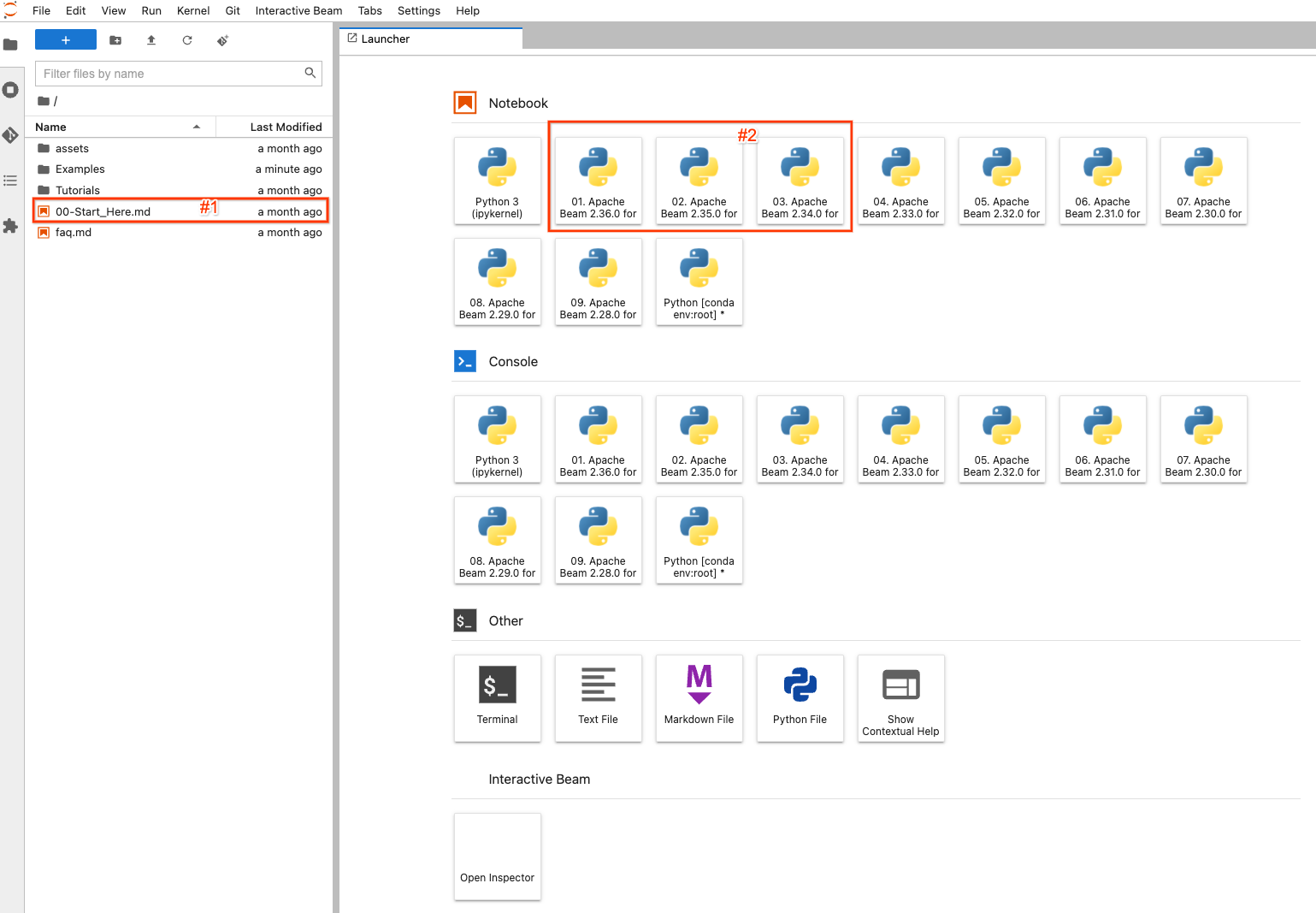
On the left side, there is a file explorer to view examples, tutorials and assets on the notebook instance. To easily navigate the files, you may double-click the 00-Start_Here.md (#1 in the screenshot) file to view detailed information about the files.

On the right side, it displays the default launcher page of JupyterLab. To create and open a completely new notebook file and code with a selected version of Apache Beam, click one of (#2) the items with Apache Beam >=2.34.0 (because beam_sql was introduced in 2.34.0) installed.

Create/open a notebook

For example, if you clicked the image button with Apache Beam 2.36.0, you would see an Untitled.ipynb file created and opened.

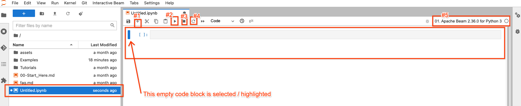
In the file explorer, your new notebook file has been created as Untitled.ipynb.

On the right side, in the opened notebook, there are 4 buttons on top that you may interact most frequently with:

• #1: insert an empty code block after the selected / highlighted code block
• #2: execute the code in the block that is selected / highlighted
• #3: interrupt code execution if your code execution is stuck
• #4: “Restart the kernel”: clear all states from code executions and start from fresh

There is a button on the top-right (#5) for you to choose a different Apache Beam version if needed, so it’s not set in stone.

You can always double-click a file from the file explorer to open it without creating a new one.

Beam SQL

beam_sql magic

beam_sql is an IPython custom magic. If you’re not familiar with magics, here are some built-in examples. It’s a convenient way to validate your queries locally against known/test data sources when prototyping a Beam pipeline with SQL, before productionizing it on remote cluster/services.

The Apache Beam Notebooks environment has preloaded the beam_sql magic and basic apache-beam modules so you can directly use them without additional imports. You can also explicitly load the magic via %load_ext apache_beam.runners.interactive.sql.beam_sql_magics and apache-beam modules if you set up your own notebook elsewhere.

You can type:

%beam_sql -h

and then execute the code to learn how to use the magic:

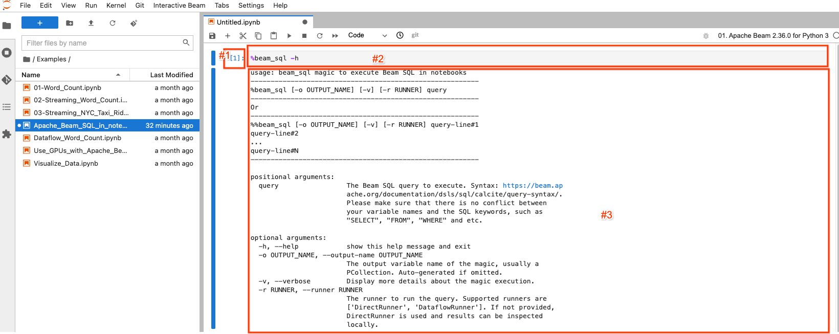
The selected/highlighted block is called a notebook cell. It mainly has 3 components:

• #1: The execution count. [1] indicates this block is the first executed code. It increases by 1 for each piece of code you execute even if you re-execute the same piece of code. [ ] indicates this block is not executed.
• #2: The cell input: the code gets executed.
• #3: The cell output: the output of the code execution. Here it contains the help documentation of the beam_sql magic.

Create a PCollection

There are 3 scenarios for Beam SQL when creating a PCollection:

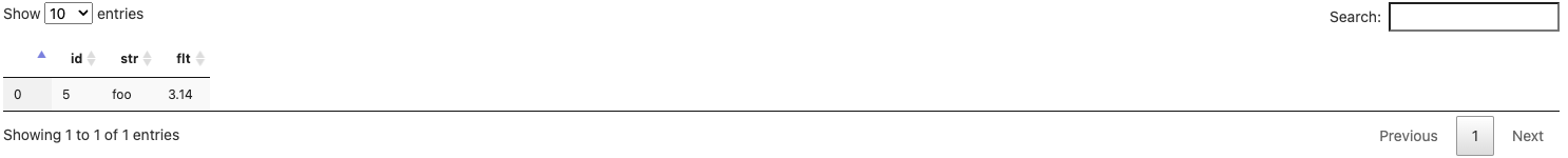
1. Use Beam SQL to create a PCollection from constant values

%%beam_sql -o pcoll
SELECT CAST(1 AS INT) AS id, CAST('foo' AS VARCHAR) AS str, CAST(3.14 AS DOUBLE) AS flt

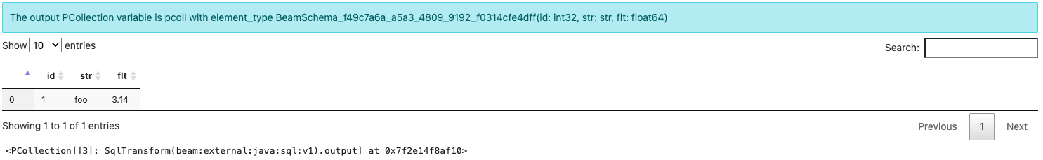
The beam_sql magic creates and outputs a PCollection named pcoll with element_type like BeamSchema_...(id: int32, str: str, flt: float64).

Note that you have not explicitly created a Beam pipeline. You get a PCollection because the beam_sql magic always implicitly creates a pipeline to execute your SQL query. To hold the elements with each field’s type info, Beam automatically creates a schema as the element_type for the created PCollection. You will learn more about schema-aware PCollections later.

2. Use Beam SQL to query a PCollection

You can chain another SQL using the output from a previous SQL (or any schema-aware PCollection produced by any normal Beam PTransforms) as the input to produce a new PCollection.

Note: if you name the output PCollection, make sure that it’s unique in your notebook to avoid overwriting a different PCollection.

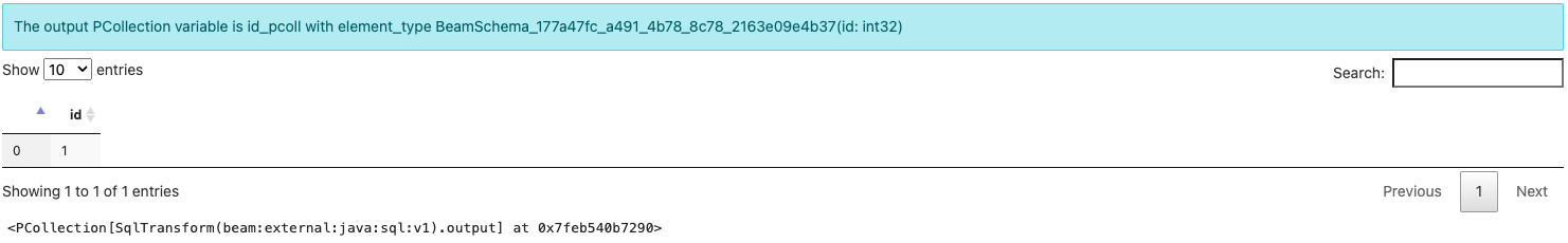
%%beam_sql -o id_pcoll
SELECT id FROM pcoll

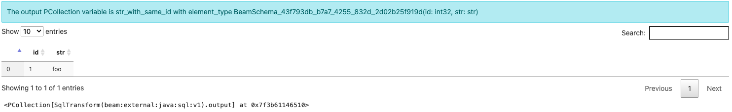
3. Use Beam SQL to join multiple PCollections

You can query multiple PCollections from a single query.

%%beam_sql -o str_with_same_id
SELECT id, str FROM pcoll JOIN id_pcoll USING (id)

Now you have learned how to use the beam_sql magic to create PCollections and inspect their results.

Tip: if you accidentally delete some of the notebook cell outputs, you can always check the content of a PCollection by invoking ib.show(pcoll_name) or ib.collect(pcoll_name) where ib stands for “Interactive Beam” (learn more).

Schema-aware PCollections

The beam_sql magic provides the flexibility to seamlessly mix SQL and non-SQL Beam statements to build pipelines and even run them on Dataflow. However, each PCollection queried by Beam SQL needs to have a schema. For the beam_sql magic, it’s recommended to use typing.NamedTuple when a schema is desired. You can go through the below example to learn more details about schema-aware PCollections.

Setup

In the setup of this example, you will:

• Install PyPI package names using the built-in %pip magic: you will use the module to generate some random English names as the raw data input.
• Define a schema with NamedTuple that has 2 attributes: id - an unique numeric identifier of a person; name - a string name of a person.
• Define a pipeline with an InteractiveRunner to utilize notebook related features of Apache Beam.

%pip install names

import names
from typing import NamedTuple

class Person(NamedTuple):
    id: int
    name: str

p = beam.Pipeline(InteractiveRunner())

There is no visible output for the code execution.

Create schema-aware PCollections without using SQL

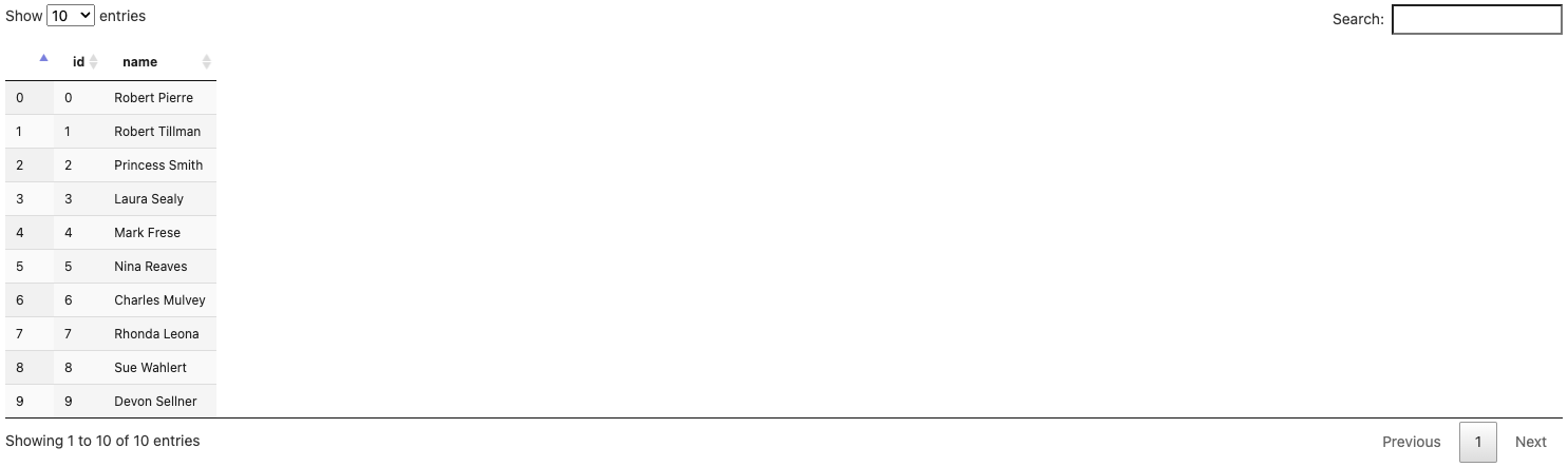
persons = (p
           | beam.Create([Person(id=x, name=names.get_full_name()) for x in range(10)]))
ib.show(persons)

persons_2 = (p
             | beam.Create([Person(id=x, name=names.get_full_name()) for x in range(5, 15)]))
ib.show(persons_2)

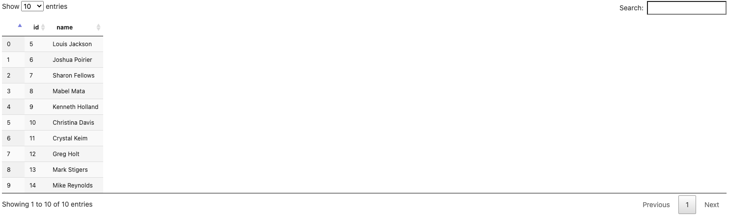
Now you have 2 PCollections both with the same schema defined by the Person class:

• persons contains 10 records for 10 persons with ids ranging from 0 to 9,
• persons_2 contains another 10 records for 10 persons with ids ranging from 5 to 14.

Encode and Decode of schema-aware PCollections

For this example, you still need one more piece of data from the first pcoll that you have created with instructions in this post.

You can use the original pcoll. Optionally, if you want to exercise using coders explicitly with schema-aware PCollections, you can add a Text I/O into the mix: write the content of pcoll into a text file retaining its schema information, then read the file back into a new schema-aware PCollection called pcoll_in_file, and use the new PCollection to join persons and persons_2 to find names with the common id in all three of them.

To encode pcoll into a file, execute:

coder=beam.coders.registry.get_coder(pcoll.element_type)
pcoll | beam.io.textio.WriteToText('/tmp/pcoll', coder=coder)
pcoll.pipeline.run().wait_until_finish()

!cat /tmp/pcoll*

The above code execution writes the PCollection pcoll (basically {id: 1, str: foo, flt: 3.14}) into a text file using the coder assigned by Beam. As you can see, the file content is recorded in a binary non human-readable format, and that’s normal.

To decode the file content into a new PCollection, execute:

pcoll_in_file = p | beam.io.ReadFromText(
    '/tmp/pcoll*', coder=coder).with_output_types(
    pcoll.element_type)

ib.show(pcoll_in_file)

Note you have to use the same coder during encoding and decoding, and furthermore you may assign the schema explicitly to the new PCollection through with_output_types().

Reading out the encoded binary content from the text file and decoding it with the correct coder, the content of pcoll is recovered into pcoll_in_file. You can use this technique to save and share your data through any Beam I/O (not necessarily a text file) with collaborators who work on their own pipelines (not just in your notebook session or pipelines).

Schema in beam_sql magic

The beam_sql magic automatically registers a RowCoder for your NamedTuple schema so that you only need to focus on preparing your data for query without worrying about coders. To see more verbose details of what the beam_sql magic does behind the scenes, you can use the -v option.

For example, you can look for all elements with id < 5 in persons with the below query and assign the output to persons_id_lt_5.

%%beam_sql -o persons_id_lt_5 -v
SELECT * FROM persons WHERE id < 5

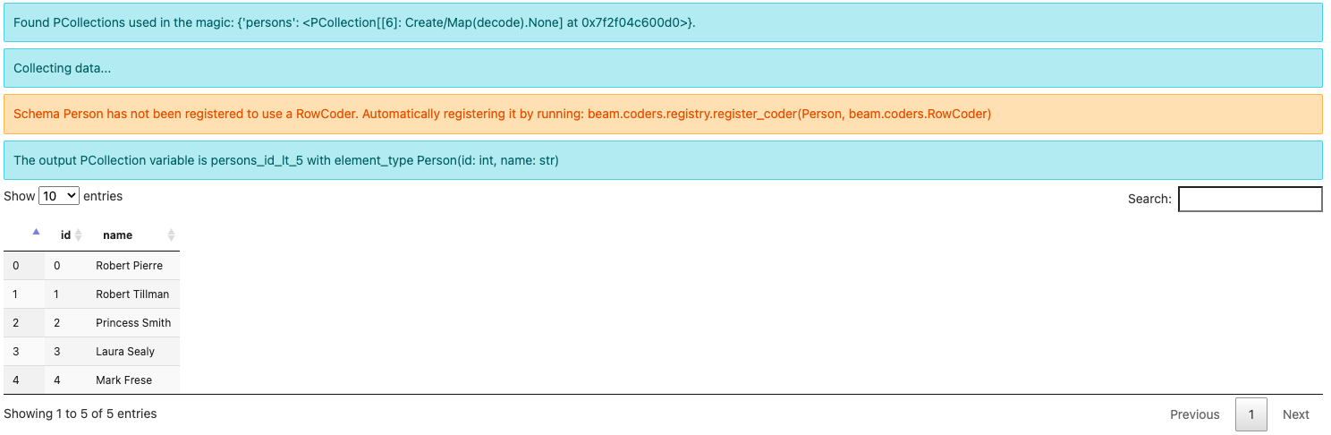
Since this is the first time running this query, you might see a warning message about:

Schema Person has not been registered to use a RowCoder. Automatically registering it by running: beam.coders.registry.register_coder(Person, beam.coders.RowCoder)

The beam_sql magic helps registering a RowCoder for each schema you define and use whenever it finds one. You can also explicitly run the same code to do so.

Note the output element type is Person(id: int, name: str) instead of BeamSchema_… because you have selected all the fields from a single PCollection of the known type Person(id: int, name: str).

Another example, you can query for all names from persons and persons_2 with the same ids and assign the output to persons_with_common_id:

%%beam_sql -o persons_with_common_id -v
SELECT * FROM persons JOIN persons_2 USING (id)

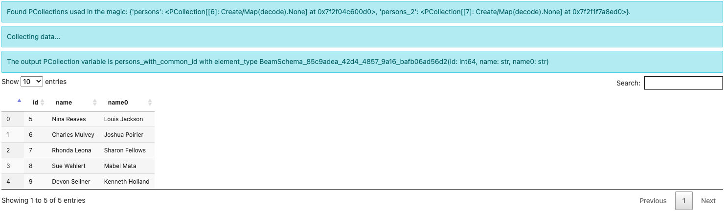
Note the output element type is now some BeamSchema_...(id: int64, name: str, name0: str). Because you have selected columns from both PCollections, there is no known schema to hold the result. Beam automatically creates a schema and differentiates the conflicted field name by suffixing 0 to one of them.

And since Person is already previously registered with a RowCoder, there is no more warning about registering it even with the -v option.

Additionally, you can do a join with pcoll_in_file, persons and persons_2:

%%beam_sql -o entry_with_common_id

SELECT pcoll_in_file.id, persons.name AS name_1, persons_2.name AS name_2
FROM pcoll_in_file JOIN persons ON pcoll_in_file.id = persons.id
JOIN persons_2 ON pcoll_in_file.id = persons_2.id

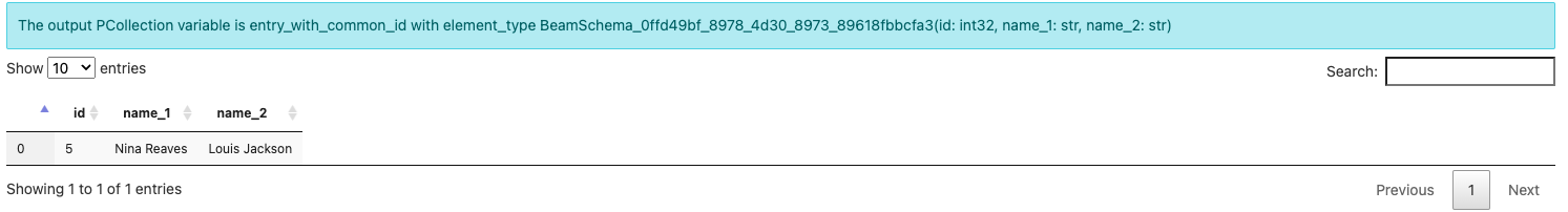
The schema generated reflects the column renaming you have done in the SQL.

An Example

You will go through an example to find out the US state with the most COVID positive cases on a specific day with data provided by the covid tracking project.

Get the data

import json
import requests

# The covidtracking project has stopped collecting new data, current data ends on 2021-03-07
json_current='https://api.covidtracking.com/v1/states/current.json'

def get_json_data(url):
  with requests.Session() as session:
    data = json.loads(session.get(url).text)
  return data

current_data = get_json_data(json_current)

current_data[0]

The data is dated as 2021-03-07. It contains many details about COVID cases for different states in the US. current_data[0] is just one of the data points.

You can get rid of most of the columns of the data. For example, just focus on “date”, “state”, “positive” and “negative”, and then define a schema UsCovidData:

from typing import Optional

class UsCovidData(NamedTuple):
    partition_date: str  # Remember to str(e['date']).
    state: str
    positive: int
    negative: Optional[int]

Note:

• date is a keyword in (Calcite)SQL, use a different field name such as partition_date;
• date from the data is an int type, not str. Make sure you convert the data using str() or use date: int.
• negative has missing values and the default is None. So instead of negative: int, it should be negative: Optional[int]. Or you can convert None into 0 when using the schema.

Then parse the json data into a PCollection with the schema:

p_sql = beam.Pipeline(runner=InteractiveRunner())
covid_data = (p_sql
        | 'Create PCollection from json' >> beam.Create(current_data)
        | 'Parse' >> beam.Map(
            lambda e: UsCovidData(
                partition_date=str(e['date']),
                state=e['state'],
                positive=e['positive'],
                negative=e['negative'])).with_output_types(UsCovidData))
ib.show(covid_data)

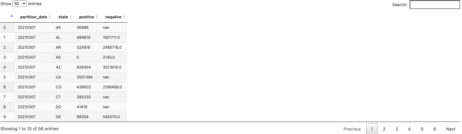
Query

You can now find the biggest positive on the “current day” (2021-03-07).

%%beam_sql -o max_positive
SELECT partition_date, MAX(positive) AS positive
FROM covid_data
GROUP BY partition_date

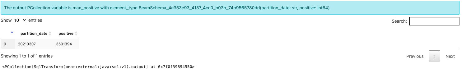
However, this is just the positive number. You cannot observe the state that has this maximum number nor the negative case number for the state.

To enrich your result, you have to join this data back to the original data set you have parsed.

%%beam_sql -o entry_with_max_positive
SELECT covid_data.partition_date, covid_data.state, covid_data.positive, {fn IFNULL(covid_data.negative, 0)} AS negative
FROM covid_data JOIN max_positive
USING (partition_date, positive)

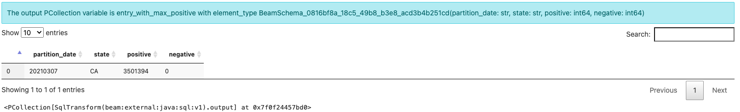
Now you can see all columns of the data with the maximum positive case on 2021-03-07. Note: to handle missing values of the negative column in the original data, you can use {fn IFNULL(covid_data.negative, 0)} to set null values to 0.

When you’re ready to scale up, you can translate the SQLs into a pipeline with SqlTransforms and run your pipeline on a distributed runner like Flink or Spark. This post demonstrates it by launching a one-shot job on Dataflow from the notebook with the help of beam_sql magic.

Run on Dataflow

Now that you have a pipeline that parses US COVID data from json to find positive/negative/state information for the state with the most positive cases on each day, you can try applying it to all historical daily data and running it on Dataflow.

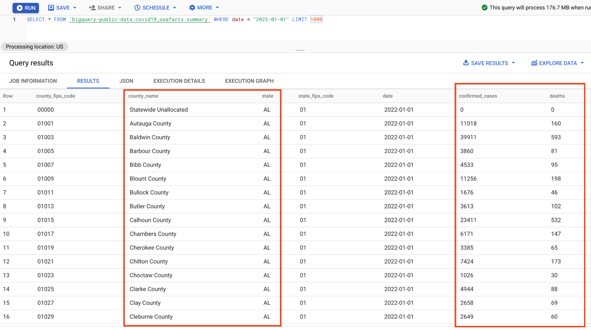
The new data source you will use is a public dataset from USAFacts US Coronavirus Database that contains all historical daily summary of COVID cases in the US.

The schema of data is very similar to what the covid tracking project website provides. The fields you will query are: date, state, confirmed_cases, and deaths.

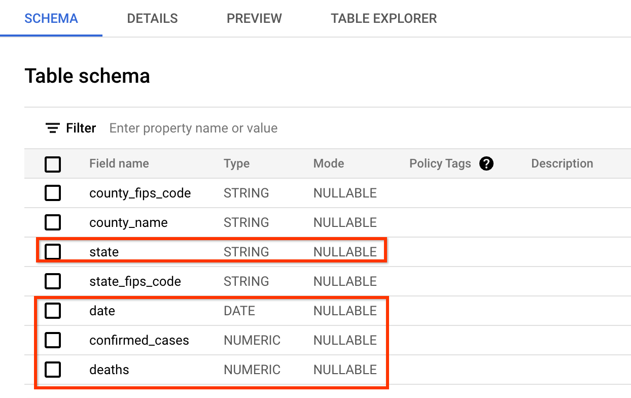
A preview of the data looks like below (you may skip the inspection in BigQuery and just take a look at the screenshot):

The format of the data is slightly different from the json data you parsed in the previous pipeline because the numbers are grouped by counties instead of states, thus some additional aggregations need to be done in the SQLs.

If you need a fresh execution, you may click the “Restart the kernel” button on the top menu.

Full code is as below, on-top of the original pipeline and queries:

• It changes the source from a single-day data to a more complete historical data;
• It changes the I/O and schema to accommodate the new dataset;
• It changes the SQLs to include more aggregations to accommodate the new format of the dataset.

Prepare the data with schema

from typing import NamedTuple
from typing import Optional

# Public BQ dataset.
table = 'bigquery-public-data:covid19_usafacts.summary'
# Replace with your project.
project = 'YOUR-PROJECT-NAME-HERE'
# Replace with your GCS bucket.
gcs_location = 'gs://YOUR_GCS_BUCKET_HERE'

class UsCovidData(NamedTuple):
    partition_date: str
    state: str
    confirmed_cases: Optional[int]
    deaths: Optional[int]


p_on_dataflow = beam.Pipeline(runner=InteractiveRunner())
covid_data = (p_on_dataflow
        | 'Read dataset' >> beam.io.ReadFromBigQuery(
            project=project, table=table, gcs_location=gcs_location)
        | 'Parse' >> beam.Map(
            lambda e: UsCovidData(
                partition_date=str(e['date']),
                state=e['state'],
                confirmed_cases=int(e['confirmed_cases']),
                deaths=int(e['deaths']))).with_output_types(UsCovidData))

Run on Dataflow

To run SQL on Dataflow is very simple, you just need to add the option -r DataflowRunner.

%%beam_sql -o data_by_state -r DataflowRunner
SELECT partition_date, state, SUM(confirmed_cases) as confirmed_cases, SUM(deaths) as deaths
FROM covid_data
GROUP BY partition_date, state

Different from previous beam_sql magic executions, you won’t see the result immediately. Instead, a form like below is printed in the notebook cell output:

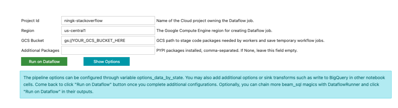
The beam_sql magic tries its best to guess your project id and preferred cloud region. You still have to input additional information necessary to submit a Dataflow job, such as a GCS bucket to stage the Dataflow job and any additional Python dependencies the job needs.

For now, ignore the form in the cell output, because you still need 2 more SQLs to: 1) find the maximum confirmed cases on each day; 2) join the maximum case data with the full data_by_state. The beam_sql magic allows you to chain SQLs, so chain 2 more by executing:

%%beam_sql -o max_cases -r DataflowRunner
SELECT partition_date, MAX(confirmed_cases) as confirmed_cases
FROM data_by_state
GROUP BY partition_date

And

%%beam_sql -o data_with_max_cases -r DataflowRunner
SELECT data_by_state.partition_date, data_by_state.state, data_by_state.confirmed_cases, data_by_state.deaths
FROM data_by_state JOIN max_cases
USING (partition_date, confirmed_cases)

By default, when running beam_sql on Dataflow, the output PCollection will be written to a text file on GCS. The “write” is automatically provided by beam_sql and mainly for your inspection of the output data for this one-shot Dataflow job. It’s lightweight and does not encode elements for further development. To save the output and share it with others, you can add more Beam I/Os into the mix.

For example, you can appropriately encode elements into text files using the technique described in the above schema-aware PCollections example.

from apache_beam.options.pipeline_options import GoogleCloudOptions

coder = beam.coders.registry.get_coder(data_with_max_cases.element_type)
max_data_file = gcs_location + '/encoded_max_data'
data_with_max_cases | beam.io.textio.WriteToText(max_data_file, coder=coder)

Furthermore, you can create a new BQ dataset in your own project to store the processed data.

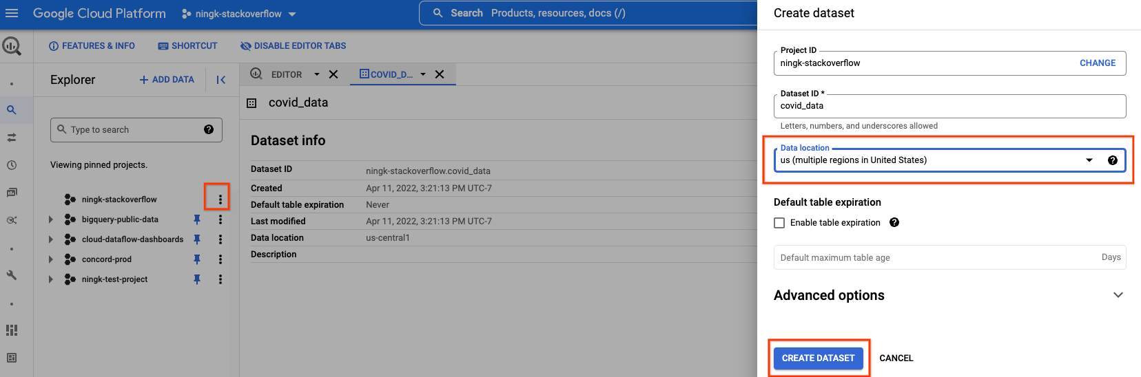
You have to select the same data location as the public BigQuery data you are reading. In this case, “us (multiple regions in United States)”.

Once you finish creating an empty dataset, you can execute below:

output_table=f'{project}:covid_data.max_analysis'
bq_schema = {
    'fields': [
        {'name': 'partition_date', 'type': 'STRING'},
        {'name': 'state', 'type': 'STRING'},
        {'name': 'confirmed_cases', 'type': 'INTEGER'},
        {'name': 'deaths', 'type': 'INTEGER'}]}
(data_with_max_cases
  | 'To json-like' >> beam.Map(lambda x: {
      'partition_date': x.partition_date,
      'state': x.state,
      'confirmed_cases': x.confirmed_cases,
      'deaths': x.deaths})
  | beam.io.WriteToBigQuery(
      table=output_table,
      schema=bq_schema,
      method='STREAMING_INSERTS',
      custom_gcs_temp_location=gcs_location))

Now back in the form of the last SQL cell output, you may fill in necessary information to run the pipeline on Dataflow. An example input looks like below:

Because this pipeline doesn’t use any additional Python dependency, “Additional Packages” is left empty. In the previous example where you have installed a package called names, to run that pipeline on Dataflow, you have to put names in this field.

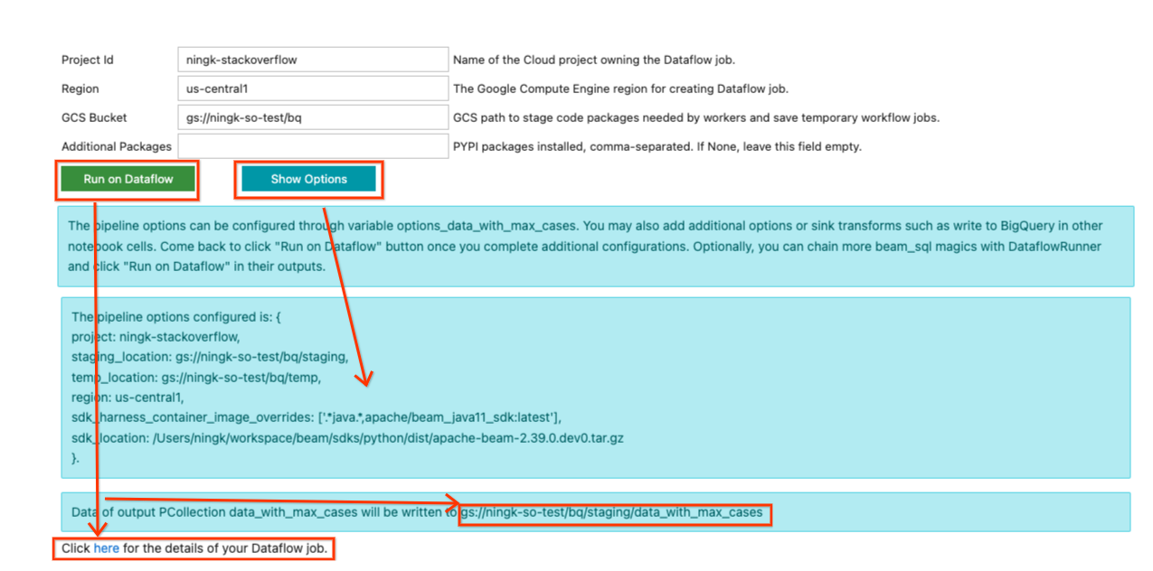
Once you finish updating your inputs, you can click the Show Options button to view what pipeline options have been configured based on your inputs. A variable options_[YOUR_OUTPUT_PCOLL_NAME] is generated, and you can supply more pipeline options to it if the form is not enough for your execution.

Once you are ready to submit the Dataflow job, click the Run on Dataflow button. It tells you where the default output would be written, and after a while, a line with:

Click here for the details of your Dataflow job.

would be displayed. You can click on the hyperlink to go to your Dataflow job page. (Optionally, you can ignore the form and continue development to extend your pipeline. Once you are satisfied with the state of your pipeline, you can come back to the form and submit the job to Dataflow.)

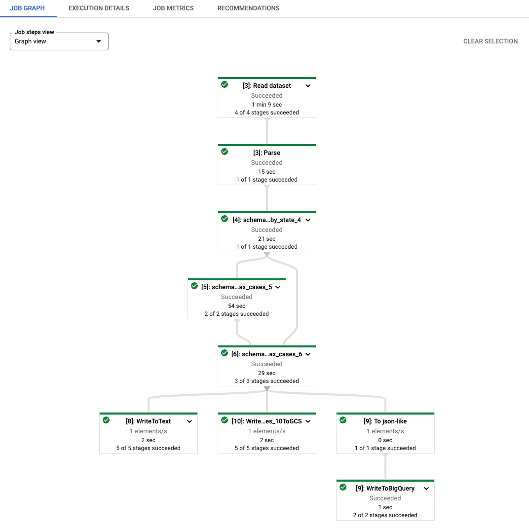
As you can see, each transform name of the generated Dataflow job is prefixed with a string [number]: . This is to distinguish re-executed codes in notebooks because Beam requires each transform to have a distinct name. Under the hood, the beam_sql magic also stages your schema information to Dataflow, so you might see transforms named as schema_loaded_beam_sql_…. This is because the NamedTuple defined in the notebook is likely in the __main__ scope and Dataflow is not aware of them at all. To minimize user intervention and avoid pickling the whole main session (and it’s infeasible to pickle the main session when it contains unpickle-able attributes), the beam_sql magic optimizes the staging process by serializing your schemas, staging them to Dataflow, and then deserialize/load them for job execution.

Once the job succeeds, the result of the output PCollection would be written to places instructed by your I/O transforms. Note: running beam_sql on Dataflow generates a one-shot job and it’s not interactive.

A simple inspection of the data from the default output location:

!gsutil cat 'gs://ningk-so-test/bq/staging/data_with_max_cases*'

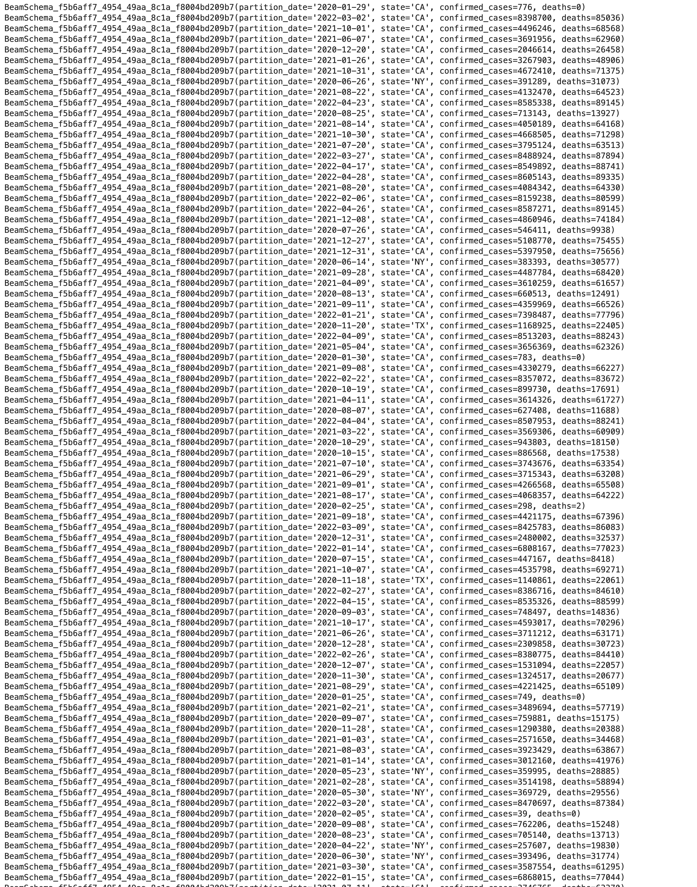
The text file with encoded binary data written by your WriteToText:

!gsutil cat 'gs://ningk-so-test/bq/encoded_max_data*'

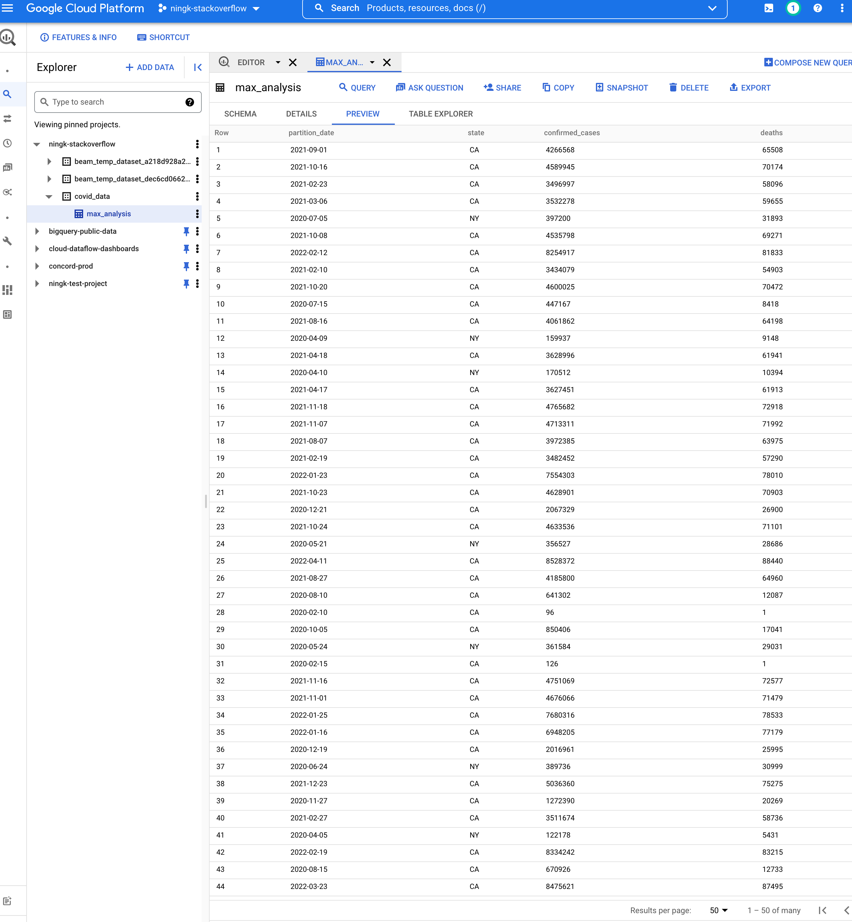
The table YOUR-PROJECT:covid_data.max_analysis created by your WriteToBigQuery:

Run on other OSS runners directly with the beam_sql magic

On the day this blog is posted, the beam_sql magic only supports DirectRunner (interactive) and DataflowRunner (one-shot). It’s a simple wrapper on top of the SqlTransform with interactive input widgets implemented by ipywidgets. You can implement your own runner support or utilities by following the instructions.

Additionally, support for other OSS runners are WIP, for example, support using FlinkRunner with the beam_sql magic.

Conclusions

The beam_sql magic and Apache Beam Notebooks combined is a convenient tool for you to learn Beam SQL and mix Beam SQL into prototyping and productionizing ( e.g., to Dataflow) your Beam pipelines with minimum setups.

For more details about the Beam SQL syntax, check out the Beam Calcite SQL compatibility and the Apache Calcite SQL syntax.