Beam lets you process unbounded, out-of-order, global-scale data with portable high-level pipelines. Stateful processing is a new feature of the Beam model that expands the capabilities of Beam, unlocking new use cases and new efficiencies. In this post, I will guide you through stateful processing in Beam: how it works, how it fits in with the other features of the Beam model, what you might use it for, and what it looks like in code.

Note: This post has been updated in May of 2019, to include Python snippets!

Warning: new features ahead!: This is a very new aspect of the Beam model. Runners are still adding support. You can try it out today on multiple runners, but do check the runner capability matrix for the current status in each runner.

First, a quick recap: In Beam, a big data processing pipeline is a directed, acyclic graph of parallel operations called PTransforms processing data from PCollections. I’ll expand on that by walking through this illustration:

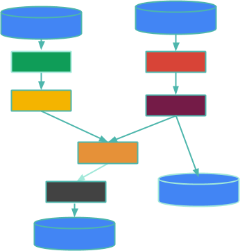
The boxes are PTransforms and the edges represent the data in PCollections flowing from one PTransform to the next. A PCollection may be bounded (which means it is finite and you know it) or unbounded (which means you don’t know if it is finite or not - basically, it is like an incoming stream of data that may or may not ever terminate). The cylinders are the data sources and sinks at the edges of your pipeline, such as bounded collections of log files or unbounded data streaming over a Kafka topic. This blog post isn’t about sources or sinks, but about what happens in between - your data processing.

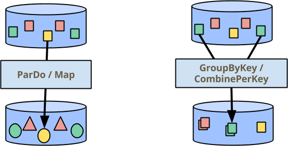
There are two main building blocks for processing your data in Beam: ParDo, for performing an operation in parallel across all elements, and GroupByKey (and the closely related CombinePerKey that I will talk about quite soon) for aggregating elements to which you have assigned the same key. In the picture below (featured in many of our presentations) the color indicates the key of the element. Thus the GroupByKey/CombinePerKey transform gathers all the green squares to produce a single output element.

But not all use cases are easily expressed as pipelines of simple ParDo/Map and GroupByKey/CombinePerKey transforms. The topic of this blog post is a new extension to the Beam programming model: per-element operation augmented with mutable state.

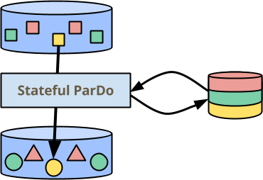
In the illustration above, ParDo now has a bit of durable, consistent state on the side, which can be read and written during the processing of each element. The state is partitioned by key, so it is drawn as having disjoint sections for each color. It is also partitioned per window, but I thought plaid would be a bit much :-). I’ll talk about why state is partitioned this way a bit later, via my first example.

For the rest of this post, I will describe this new feature of Beam in detail - how it works at a high level, how it differs from existing features, how to make sure it is still massively scalable. After that introduction at the model level, I’ll walk through a simple example of how you use it in the Beam Java SDK.

How does stateful processing in Beam work?

The processing logic of your ParDo transform is expressed through the DoFn that it applies to each element. Without stateful augmentations, a DoFn is a mostly-pure function from inputs to one or more outputs, corresponding to the Mapper in a MapReduce. With state, a DoFn has the ability to access persistent mutable state while processing each input element. Consider this illustration:

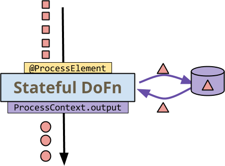
The first thing to note is that all the data - the little squares, circles, and triangles - are red. This is to illustrate that stateful processing occurs in the context of a single key - all of the elements are key-value pairs with the same key. Calls from your chosen Beam runner to the DoFn are colored in yellow, while calls from the DoFn to the runner are in purple:

• The runner invokes the DoFn’s @ProcessElement method on each element for a key+window.
• The DoFn reads and writes state - the curved arrows to/from the storage on the side.
• The DoFn emits output (or side output) to the runner as usual via ProcessContext.output (resp. ProcessContext.sideOutput).

At this very high level, it is pretty intuitive: In your programming experience, you have probably at some point written a loop over elements that updates some mutable variables while performing other actions. The interesting question is how does this fit into the Beam model: how does it relate with other features? How does it scale, since state implies some synchronization? When should it be used versus other features?

How does stateful processing fit into the Beam model?

To see where stateful processing fits in the Beam model, consider another way that you can keep some “state” while processing many elements: CombineFn. In Beam, you can write Combine.perKey(CombineFn) in Java or Python to apply an associative, commutative accumulating operation across all the elements with a common key (and window).

Here is a diagram illustrating the basics of a CombineFn, the simplest way that a runner might invoke it on a per-key basis to build an accumulator and extract an output from the final accumulator:

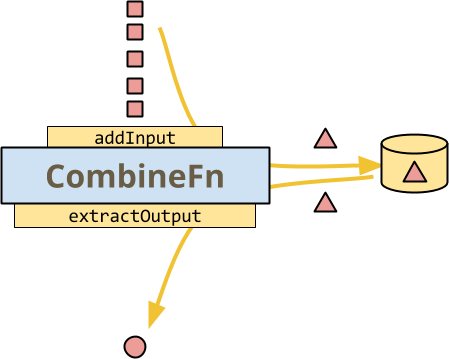
As with the illustration of stateful DoFn, all the data is colored red, since this is the processing of Combine for a single key. The illustrated method calls are colored yellow, since they are all controlled by the runner: The runner invokes addInput on each method to add it to the current accumulator.

• The runner persists the accumulator when it chooses.
• The runner calls extractOutput when ready to emit an output element.

At this point, the diagram for CombineFn looks a whole lot like the diagram for stateful DoFn. In practice, the flow of data is, indeed, quite similar. But there are important differences, even so:

• The runner controls all invocations and storage here. You do not decide when or how state is persisted, when an accumulator is discarded (based on triggering) or when output is extracted from an accumulator.
• You can only have one piece of state - the accumulator. In a stateful DoFn you can read only what you need to know and write only what has changed.
• You don’t have the extended features of DoFn, such as multiple outputs per input or side outputs. (These could be simulated by a sufficient complex accumulator, but it would not be natural or efficient. Some other features of DoFn such as side inputs and access to the window make perfect sense for CombineFn)

But the main thing that CombineFn allows a runner to do is to mergeAccumulators, the concrete expression of the CombineFn’s associativity. This unlocks some huge optimizations: the runner can invoke multiple instances of a CombineFn on a number of inputs and later combine them in a classic divide-and-conquer architecture, as in this picture:

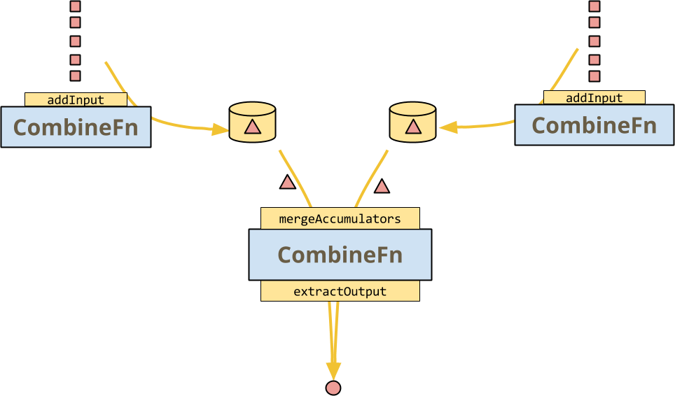
The contract of a CombineFn is that the result should be exactly the same, whether or not the runner decides to actually do such a thing, or even more complex trees with hot-key fanout, etc.

This merge operation is not (necessarily) provided by a stateful DoFn: the runner cannot freely branch its execution and recombine the states. Note that the input elements are still received in an arbitrary order, so the DoFn should be insensitive to ordering and bundling but it doesn’t mean the output must be exactly equal. (fun and easy fact: if the outputs are actually always equal, then the DoFn is an associative and commutative operator)

So now you can see how a stateful DoFn differs from CombineFn, but I want to step back and extrapolate this to a high level picture of how state in Beam relates to using other features to achieve the same or similar goals: In a lot of cases, what stateful processing represents is a chance to “get under the hood” of the highly abstract mostly-deterministic functional paradigm of Beam and do potentially-nondeterministic imperative-style programming that is hard to express any other way.

Example: arbitrary-but-consistent index assignment

Suppose that you want to give an index to every incoming element for a key-and-window. You don’t care what the indices are, just as long as they are unique and consistent. Before diving into the code for how to do this in a Beam SDK, I’ll go over this example from the level of the model. In pictures, you want to write a transform that maps input to output like this:

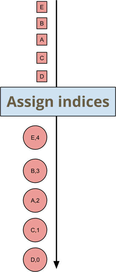
The order of the elements A, B, C, D, E is arbitrary, hence their assigned indices are arbitrary, but downstream transforms just need to be OK with this. There is no associativity or commutativity as far as the actual values are concerned. The order-insensitivity of this transform only extends to the point of ensuring the necessary properties of the output: no duplicated indices, no gaps, and every element gets an index.

Conceptually expressing this as a stateful loop is as trivial as you can imagine: The state you should store is the next index.

• As an element comes in, output it along with the next index.
• Increment the index.

This presents a good opportunity to talk about big data and parallelism, because the algorithm in those bullet points is not parallelizable at all! If you wanted to apply this logic over an entire PCollection, you would have to process each element of the PCollection one-at-a-time… this is obviously a bad idea. State in Beam is tightly scoped so that most of the time a stateful ParDo transform should still be possible for a runner to execute in parallel, though you still have to be thoughtful about it.

A state cell in Beam is scoped to a key+window pair. When your DoFn reads or writes state by the name of "index", it is actually accessing a mutable cell specified by "index" along with the key and window currently being processed. So, when thinking about a state cell, it may be helpful to consider the full state of your transform as a table, where the rows are named according to names you use in your program, like "index", and the columns are key+window pairs, like this:

(if you have a superb spatial sense, feel free to imagine this as a cube where keys and windows are independent dimensions)

You can provide the opportunity for parallelism by making sure that table has enough columns. You might have many keys and many windows, or you might have many of just one or the other:

• Many keys in few windows, for example a globally windowed stateful computation keyed by user ID.
• Many windows over few keys, for example a fixed windowed stateful computation over a global key.

Caveat: all Beam runners today parallelize only over the key.

Most often your mental model of state can be focused on only a single column of the table, a single key+window pair. Cross-column interactions do not occur directly, by design.

State in Beam’s Java SDK

Now that I have talked a bit about stateful processing in the Beam model and worked through an abstract example, I’d like to show you what it looks like to write stateful processing code using Beam’s Java SDK. Here is the code for a stateful DoFn that assigns an arbitrary-but-consistent index to each element on a per key-and-window basis:

new DoFn<KV<MyKey, MyValue>, KV<Integer, KV<MyKey, MyValue>>>() {

  // A state cell holding a single Integer per key+window
  @StateId("index")
  private final StateSpec<ValueState<Integer>> indexSpec =
      StateSpecs.value(VarIntCoder.of());

  @ProcessElement
  public void processElement(
      ProcessContext context,
      @StateId("index") ValueState<Integer> index) {
    int current = firstNonNull(index.read(), 0);
    context.output(KV.of(current, context.element()));
    index.write(current+1);
  }
}

class IndexAssigningStatefulDoFn(DoFn):
  INDEX_STATE = CombiningStateSpec('index', sum)

  def process(self, element, index=DoFn.StateParam(INDEX_STATE)):
    unused_key, value = element
    current_index = index.read()
    yield (value, current_index)
    index.add(1)

Let’s dissect this:

• The first thing to look at is the presence of a couple of @StateId("index") annotations. This calls out that you are using a mutable state cell named “index” in this DoFn. The Beam Java SDK, and from there your chosen runner, will also note these annotations and use them to wire up your DoFn correctly.
• The first @StateId("index") is annotated on a field of type StateSpec (for “state specification”). This declares and configures the state cell. The type parameter ValueState describes the kind of state you can get out of this cell - ValueState stores just a single value. Note that the spec itself is not a usable state cell - you need the runner to provide that during pipeline execution.
• To fully specify a ValueState cell, you need to provide the coder that the runner will use (as necessary) to serialize the value you will be storing. This is the invocation StateSpecs.value(VarIntCoder.of()).
• The second @StateId("index") annotation is on a parameter to your @ProcessElement method. This indicates access to the ValueState cell that was specified earlier.
• The state is accessed in the simplest way: read() to read it, and write(newvalue) to write it.
• The other features of DoFn are available in the usual way - such as context.output(...). You can also use side inputs, side outputs, gain access to the window, etc.

A few notes on how the SDK and runners see this DoFn:

• Your state cells are all explicitly declared so a Beam SDK or runner can reason about them, for example to clear them out when a window expires.
• If you declare a state cell and then use it with the wrong type, the Beam Java SDK will catch that error for you.
• If you declare two state cells with the same ID, the SDK will catch that, too.
• The runner knows that this is a stateful DoFn and may run it quite differently, for example by additional data shuffling and synchronization in order to avoid concurrent access to state cells.

Let’s look at one more example of how to use this API, this time a bit more real-world.

Example: anomaly detection

Suppose you are feeding a stream of actions by your user into some complex model to predict some quantitative expression of the sorts of actions they take, for example to detect fraudulent activity. You will build up the model from events, and also compare incoming events against the latest model to determine if something has changed.

If you try to express the building of your model as a CombineFn, you may have trouble with mergeAccumulators. Assuming you could express that, it might look something like this:

class ModelFromEventsFn extends CombineFn<Event, Model, Model> {
    @Override
    public abstract Model createAccumulator() {
      return Model.empty();
    }

    @Override
    public abstract Model addInput(Model accumulator, Event input) {
      return accumulator.update(input); // this is encouraged to mutate, for efficiency
    }

    @Override
    public abstract Model mergeAccumulators(Iterable<Model> accumulators) {
      // ?? can you write this ??
    }

    @Override
    public abstract Model extractOutput(Model accumulator) {
      return accumulator; }
}

class ModelFromEventsFn(apache_beam.core.CombineFn):

  def create_accumulator(self):
    # Create a new empty model
    return Model()

  def add_input(self, model, input):
    return model.update(input)

  def merge_accumulators(self, accumulators):
    # Custom merging logic

  def extract_output(self, model):
    return model

Now you have a way to compute the model of a particular user for a window as Combine.perKey(new ModelFromEventsFn()). How would you apply this model to the same stream of events from which it is calculated? A standard way to do take the result of a Combine transform and use it while processing the elements of a PCollection is to read it as a side input to a ParDo transform. So you could side input the model and check the stream of events against it, outputting the prediction, like so:

PCollection<KV<UserId, Event>> events = ...

final PCollectionView<Map<UserId, Model>> userModels = events
    .apply(Combine.perKey(new ModelFromEventsFn()))
    .apply(View.asMap());

PCollection<KV<UserId, Prediction>> predictions = events
    .apply(ParDo.of(new DoFn<KV<UserId, Event>>() {

      @ProcessElement
      public void processElement(ProcessContext ctx) {
        UserId userId = ctx.element().getKey();
        Event event = ctx.element().getValue();

        Model model = ctx.sideinput(userModels).get(userId);

        // Perhaps some logic around when to output a new prediction
        … c.output(KV.of(userId, model.prediction(event))) …
      }
    }));

# Events is a collection of (user, event) pairs.
events = (p | ReadFromEventSource() | beam.WindowInto(....))

user_models = beam.pvalue.AsDict(
                  events
                  | beam.core.CombinePerKey(ModelFromEventsFn()))

def event_prediction(user_event, models):
  user = user_event[0]
  event = user_event[1]

  # Retrieve the model calculated for this user
  model = models[user]

  return (user, model.prediction(event))

# Predictions is a collection of (user, prediction) pairs.
predictions = events | beam.Map(event_prediction, user_models)

In this pipeline, there is just one model emitted by the Combine.perKey(...) per user, per window, which is then prepared for side input by the View.asMap() transform. The processing of the ParDo over events will block until that side input is ready, buffering events, and will then check each event against the model. This is a high latency, high completeness solution: The model takes into account all user behavior in the window, but there can be no output until the window is complete.

Suppose you want to get some results earlier, or don’t even have any natural windowing, but just want continuous analysis with the “model so far”, even though your model may not be as complete. How can you control the updates to the model against which you are checking your events? Triggers are the generic Beam feature for managing completeness versus latency tradeoffs. So here is the same pipeline with an added trigger that outputs a new model one second after input arrives:

PCollection<KV<UserId, Event>> events = ...

PCollectionView<Map<UserId, Model>> userModels = events

    // A tradeoff between latency and cost
    .apply(Window.triggering(
        AfterProcessingTime.pastFirstElementInPane(Duration.standardSeconds(1)))

    .apply(Combine.perKey(new ModelFromEventsFn()))
    .apply(View.asMap());

events = ...

user_models = beam.pvalue.AsDict(
                  events
                  | beam.WindowInto(GlobalWindows(),
                      trigger=trigger.AfterAll(
                          trigger.AfterCount(1),
                          trigger.AfterProcessingTime(1)))
                  | beam.CombinePerKey(ModelFromEventsFn()))

This is often a pretty nice tradeoff between latency and cost: If a huge flood of events comes in a second, then you will only emit one new model, so you won’t be flooded with model outputs that you cannot even use before they are obsolete. In practice, the new model may not be present on the side input channel until many more seconds have passed, due to caches and processing delays preparing the side input. Many events (maybe an entire batch of activity) will have passed through the ParDo and had their predictions calculated according to the prior model. If the runner gave a tight enough bound on cache expirations and you used a more aggressive trigger, you might be able to improve latency at additional cost.

But there is another cost to consider: you are outputting many uninteresting outputs from the ParDo that will be processed downstream. If the “interestingness” of the output is only well-defined relative to the prior output, then you cannot use a Filter transform to reduce data volume downstream.

Stateful processing lets you address both the latency problem of side inputs and the cost problem of excessive uninteresting output. Here is the code, using only features I have already introduced:

new DoFn<KV<UserId, Event>, KV<UserId, Prediction>>() {

  @StateId("model")
  private final StateSpec<ValueState<Model>> modelSpec =
      StateSpecs.value(Model.coder());

  @StateId("previousPrediction")
  private final StateSpec<ValueState<Prediction>> previousPredictionSpec =
      StateSpecs.value(Prediction.coder());

  @ProcessElement
  public void processElement(
      ProcessContext c,
      @StateId("previousPrediction") ValueState<Prediction> previousPredictionState,
      @StateId("model") ValueState<Model> modelState) {
    UserId userId = c.element().getKey();
    Event event = c.element().getValue()

    Model model = modelState.read();
    Prediction previousPrediction = previousPredictionState.read();
    Prediction newPrediction = model.prediction(event);
    model.add(event);
    modelState.write(model);
    if (previousPrediction == null
        || shouldOutputNewPrediction(previousPrediction, newPrediction)) {
      c.output(KV.of(userId, newPrediction));
      previousPredictionState.write(newPrediction);
    }
  }
};

class ModelStatefulFn(beam.DoFn):

  PREVIOUS_PREDICTION = BagStateSpec('previous_pred_state', PredictionCoder())
  MODEL_STATE = CombiningValueStateSpec('model_state',
                                        ModelCoder(),
                                        ModelFromEventsFn())

  def process(self,
              user_event,
              previous_pred_state=beam.DoFn.StateParam(PREVIOUS_PREDICTION),
              model_state=beam.DoFn.StateParam(MODEL_STATE)):
    user = user_event[0]
    event = user_event[1]
    model = model_state.read()
    previous_prediction = previous_pred_state.read()

    new_prediction = model.prediction(event)
    model_state.add(event)

    if (previous_prediction is None
        or self.should_output_prediction(
            previous_prediction, new_prediction)):
      previous_pred_state.clear()
      previous_pred_state.add(new_prediction)
      yield (user, new_prediction)

Let’s walk through it,

• You have two state cells declared, @StateId("model") to hold the current state of the model for a user and @StateId("previousPrediction") to hold the prediction output previously.
• Access to the two state cells by annotation in the @ProcessElement method is as before.
• You read the current model via modelState.read(). per-key-and-window, this is a model just for the UserId of the Event currently being processed.
• You derive a new prediction model.prediction(event) and compare it against the last one you output, accessed via previousPredicationState.read().
• You then update the model model.update() and write it via modelState.write(...). It is perfectly fine to mutate the value you pulled out of state as long as you also remember to write the mutated value, in the same way you are encouraged to mutate CombineFn accumulators.
• If the prediction has changed a significant amount since the last time you output, you emit it via context.output(...) and save the prediction using previousPredictionState.write(...). Here the decision is relative to the prior prediction output, not the last one computed - realistically you might have some complex conditions here.

Most of the above is just talking through Java! But before you go out and convert all of your pipelines to use stateful processing, I want to go over some considerations as to whether it is a good fit for your use case.

Performance considerations

To decide whether to use per-key-and-window state, you need to consider how it executes. You can dig into how a particular runner manages state, but there are some general things to keep in mind:

• Partitioning per-key-and-window: perhaps the most important thing to consider is that the runner may have to shuffle your data to colocate all the data for a particular key+window. If the data is already shuffled correctly, the runner may take advantage of this.
• Synchronization overhead: the API is designed so the runner takes care of concurrency control, but this means that the runner cannot parallelize processing of elements for a particular key+window even when it would otherwise be advantageous.
• Storage and fault tolerance of state: since state is per-key-and-window, the more keys and windows you expect to process simultaneously, the more storage you will incur. Because state benefits from all the fault tolerance / consistency properties of your other data in Beam, it also adds to the cost of committing the results of processing.
• Expiration of state: also since state is per-window, the runner can reclaim the resources when a window expires (when the watermark exceeds its allowed lateness) but this could mean that the runner is tracking an additional timer per key and window to cause reclamation code to execute.

Go use it!

If you are new to Beam, I hope you are now interested in seeing if Beam with stateful processing addresses your use case. If you are already using Beam, I hope this new addition to the model unlocks new use cases for you. Do check the capability matrix to see the level of support for this new model feature on your favorite backend(s).

And please do join the community at user@beam.apache.org. We’d love to hear from you.